3.7. Standardizing data

When we collect data different variables are expressed in different units or scales. Some data are recorded in naturally, meaningful units that we might be quite familiar with:

• Height of adults in cm

• Temperature in \(^{\circ}C\)

• Cost of a pint in GBP (£)

However, in many other situations, the units are less intuitive — for instance:

• scores on an IQ test marked out of 180

• height of 2-year-olds in cm

• price of hospital visit in USD ($)

A further complication occurs when we are trying to quantify how unusual a data value is when values are presented as different units

• High school grades from different countries or systems (A-levels vs IB vs Abitur vs…..)

Across all of these cases, it can be helpful to express data in standardized units, which allows us to compare values across different scales or measurements.

Two common ways of standardizing data are:

1. Convert data to Z-scores - measuring how many standard deviations a value is from the mean

2. Convert data to quantiles - expressing values in terms of their percentile position within the distribution

In this section we will review both these approaches.

Here is a video about standardizing data using centiles

%%HTML
<iframe width="560" height="315" src="https://www.youtube.com/embed/i162CImD2BI?si=AKYH2absqZ6n8WLG" title="YouTube video player" frameborder="0" allow="accelerometer; autoplay; clipboard-write; encrypted-media; gyroscope; picture-in-picture; web-share" referrerpolicy="strict-origin-when-cross-origin" allowfullscreen></iframe>

Here is a video about standardizing data using Z-Scores

%%HTML
<iframe width="560" height="315" src="https://www.youtube.com/embed/SPgQ_D0I_q4?si=YvukrU2VD6iZSTKQ" title="YouTube video player" frameborder="0" allow="accelerometer; autoplay; clipboard-write; encrypted-media; gyroscope; picture-in-picture; web-share" referrerpolicy="strict-origin-when-cross-origin" allowfullscreen></iframe>

3.7.1. Set up Python Libraries

As usual you will need to run this code block to import the relevant Python libraries

# Set-up Python libraries - you need to run this but you don't need to change it
import numpy as np
import matplotlib.pyplot as plt
import scipy.stats as stats
import pandas as pd
import seaborn as sns
sns.set_theme(style='white')
import statsmodels.api as sm
import statsmodels.formula.api as smf

3.7.2. Import a dataset to work with

Let’s look at a fictional dataset containing some body measurements for 50 individuals

data=pd.read_csv('https://raw.githubusercontent.com/jillxoreilly/StatsCourseBook_2024/main/data/BodyData.csv')
display(data)

	ID	sex	height	weight	age
0	101708	M	161	64.8	35
1	101946	F	165	68.1	42
2	108449	F	175	76.6	31
3	108796	M	180	81.0	31
4	113449	F	179	80.1	31
5	114688	M	172	74.0	42
6	119187	F	148	54.8	45
7	120679	F	160	64.0	44
8	120735	F	188	88.4	32
9	124269	F	172	74.0	29
10	124713	M	175	76.6	26
11	127076	M	180	81.0	28
12	131626	M	162	65.6	35
13	132218	M	170	72.3	29
14	132609	F	172	74.0	41
15	134660	F	159	63.2	34
16	135195	M	169	71.4	42
17	140073	F	168	70.6	34
18	140114	M	195	95.1	41
19	145185	F	157	61.6	45
20	146279	F	180	81.0	30
21	146519	F	172	74.0	34
22	151451	F	171	73.1	37
23	152597	M	172	74.0	27
24	154672	M	167	69.7	39
25	155594	F	165	68.1	25
26	158165	M	175	76.6	45
27	159457	F	176	77.4	36
28	162323	M	173	74.8	31
29	166948	M	174	75.7	28
30	168411	M	175	76.6	29
31	168574	F	163	66.4	30
32	169209	F	159	63.2	45
33	171236	F	164	67.2	34
34	172289	M	181	81.9	27
35	173925	M	189	89.3	25
36	176598	F	169	71.4	37
37	177002	F	180	81.0	36
38	178659	M	181	81.9	26
39	180992	F	177	78.3	31
40	183304	F	176	77.4	30
41	184706	M	183	83.7	40
42	185138	M	169	71.4	28
43	185223	F	170	72.3	41
44	186041	M	175	76.6	25
45	186887	M	154	59.3	26
46	187016	M	161	64.8	32
47	198157	M	180	81.0	33
48	199112	M	172	74.0	33
49	199614	F	164	67.2	31

3.7.3. Z score

A Z-score tells us how many standard deviations a particular value lies above or below the mean of its distribution. This transformation helps us understand how unusual a given value is relative to the rest of the data — regardless of the original measurement units. For example, a Z-score of +2 means the value is two standard deviations above the mean, while a score of –1.5 means it’s 1.5 standard deviations below the mean.

Let’s convert our weights to Z-scores. We will need to know the mean and standard deviation of weight:

print(data.weight.mean())
print(data.weight.std())

73.73
7.891438140058334

To give you some instinct for Z-score let’s consider some examples:

• Someone whose weight is exactly on the mean (73.73kg) will have a Z-score of 0.

• Someone whose weight is one standard deviation below the mean (65.83kg) will have a Z-score of -1 etc.

We will calculate a Z-score for each person’s weight. To do this we will create a new column in our dataframe called WeightZ. Z score is calculated as:

\[Z = \frac{X - \text{Mean}}{\text{SD}}\]

# Create a new column and put the calcualted z-scores in it
data['WeightZ'] = (data.weight - data.weight.mean())/data.weight.std()
data

	ID	sex	height	weight	age	WeightZ
0	101708	M	161	64.8	35	-1.131606
1	101946	F	165	68.1	42	-0.713431
2	108449	F	175	76.6	31	0.363685
3	108796	M	180	81.0	31	0.921252
4	113449	F	179	80.1	31	0.807204
5	114688	M	172	74.0	42	0.034214
6	119187	F	148	54.8	45	-2.398802
7	120679	F	160	64.0	44	-1.232982
8	120735	F	188	88.4	32	1.858977
9	124269	F	172	74.0	29	0.034214
10	124713	M	175	76.6	26	0.363685
11	127076	M	180	81.0	28	0.921252
12	131626	M	162	65.6	35	-1.030230
13	132218	M	170	72.3	29	-0.181209
14	132609	F	172	74.0	41	0.034214
15	134660	F	159	63.2	34	-1.334358
16	135195	M	169	71.4	42	-0.295257
17	140073	F	168	70.6	34	-0.396632
18	140114	M	195	95.1	41	2.707998
19	145185	F	157	61.6	45	-1.537109
20	146279	F	180	81.0	30	0.921252
21	146519	F	172	74.0	34	0.034214
22	151451	F	171	73.1	37	-0.079833
23	152597	M	172	74.0	27	0.034214
24	154672	M	167	69.7	39	-0.510680
25	155594	F	165	68.1	25	-0.713431
26	158165	M	175	76.6	45	0.363685
27	159457	F	176	77.4	36	0.465061
28	162323	M	173	74.8	31	0.135590
29	166948	M	174	75.7	28	0.249638
30	168411	M	175	76.6	29	0.363685
31	168574	F	163	66.4	30	-0.928855
32	169209	F	159	63.2	45	-1.334358
33	171236	F	164	67.2	34	-0.827479
34	172289	M	181	81.9	27	1.035299
35	173925	M	189	89.3	25	1.973024
36	176598	F	169	71.4	37	-0.295257
37	177002	F	180	81.0	36	0.921252
38	178659	M	181	81.9	26	1.035299
39	180992	F	177	78.3	31	0.579109
40	183304	F	176	77.4	30	0.465061
41	184706	M	183	83.7	40	1.263395
42	185138	M	169	71.4	28	-0.295257
43	185223	F	170	72.3	41	-0.181209
44	186041	M	175	76.6	25	0.363685
45	186887	M	154	59.3	26	-1.828564
46	187016	M	161	64.8	32	-1.131606
47	198157	M	180	81.0	33	0.921252
48	199112	M	172	74.0	33	0.034214
49	199614	F	164	67.2	31	-0.827479

Look down the table for some heavy and light people. Do their z-scores look like you would expect?

3.7.4. Z-score Rule of Thumb

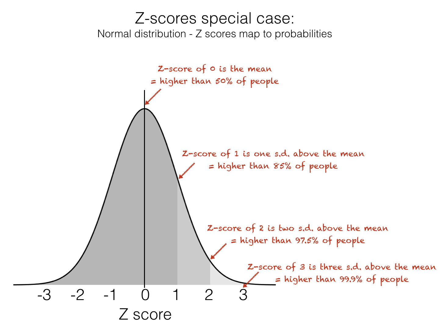
The Z-score tells us how many standard deviations above or below the mean a datapoint lies. This makes it very useful for identifying unusually high or low values within a dataset. When data is approximately normal you can easily infer a lot of information about a particular data-point based on its Z-Score. Specifically, we can use this handy rule-of-thumb to know how unusual a Z-score is:

Don’t worry if you don’t know what the Normal distribution is yet - you will learn about this in detail later in the course

• Z-Score of 0 is higher than 50% of values

• Z-Score of 1 is higher than 85% of values

• Z-Score of 2 is higher than 97.5% of values

3.7.5. Z-score Disadvantages

However, the Z-score does have a couple of disadvantages:

• The Z-score is not easily understood by non statistically trained people

• Z-scores are only meaningful if the data are approximately normally distributed, for data that are strongly skewed or contain outliers, the mean and standard deviation may not accurately reflect the typical values

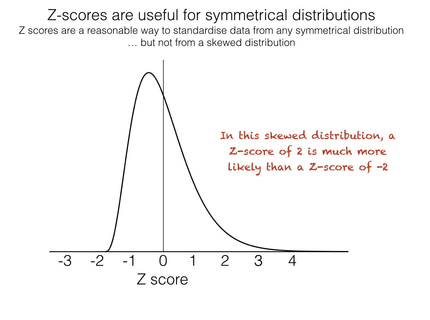
It is therefore sometimes more meaningful to standardize data by presenting them as quantiles

3.7.6. Quantiles

Quantiles (also called centiles or percentiles) tell us what proportion of data points fall below or above a given value. They’re an intuitive way to describe where a particular observation lies within a distribution.

For example, imagine my two-year-old son is 85 cm tall and 14kg. Would you say he is big for his age? You probably have no idea, because unlike adult sizes, most of us don’t have a good sense of the size distribution two-year-olds.

In fact, the two-year-old described here lies on the 25th centile for height and the 91st centile for weight, this means he is only taller than 25% of boys the same age but he weighs more than 91%.

To calculate a given quantile of a dataset we use df.quantile(), e.g., to find the 90th centile of the heights in our data set:

# find the 90th centile for height in out dataframe
data.height.quantile(q=0.9) # get 90th centile

np.float64(181.0)

The 90th centile is 181cm, ie 10% of people are taller than 181cm.

Adding quantile information to a dataset can be done using pd.qcut(), which divides the data into equal-sized groups (quantiles) and assigns each observation to one of them.

For example, we can categorize people’s weights into deciles. Deciles are 10ths, in the same way that centiles are 100ths.

• if someone’s weight in the 0th decile, that means their weight is in the bottom 10% of the sample

• if someone’s weight is in the 9th decile, it mmeans they are in the top 10% ot the sample (heavier than 90% of people)

Here we add deciles to the data frame in a new variable called weightQ:

data['weightQ'] = pd.qcut(data.weight, 10, labels = False) 
data

	ID	sex	height	weight	age	WeightZ	weightQ
0	101708	M	161	64.8	35	-1.131606	1
1	101946	F	165	68.1	42	-0.713431	2
2	108449	F	175	76.6	31	0.363685	6
3	108796	M	180	81.0	31	0.921252	7
4	113449	F	179	80.1	31	0.807204	7
5	114688	M	172	74.0	42	0.034214	4
6	119187	F	148	54.8	45	-2.398802	0
7	120679	F	160	64.0	44	-1.232982	1
8	120735	F	188	88.4	32	1.858977	9
9	124269	F	172	74.0	29	0.034214	4
10	124713	M	175	76.6	26	0.363685	6
11	127076	M	180	81.0	28	0.921252	7
12	131626	M	162	65.6	35	-1.030230	1
13	132218	M	170	72.3	29	-0.181209	3
14	132609	F	172	74.0	41	0.034214	4
15	134660	F	159	63.2	34	-1.334358	0
16	135195	M	169	71.4	42	-0.295257	3
17	140073	F	168	70.6	34	-0.396632	3
18	140114	M	195	95.1	41	2.707998	9
19	145185	F	157	61.6	45	-1.537109	0
20	146279	F	180	81.0	30	0.921252	7
21	146519	F	172	74.0	34	0.034214	4
22	151451	F	171	73.1	37	-0.079833	4
23	152597	M	172	74.0	27	0.034214	4
24	154672	M	167	69.7	39	-0.510680	2
25	155594	F	165	68.1	25	-0.713431	2
26	158165	M	175	76.6	45	0.363685	6
27	159457	F	176	77.4	36	0.465061	7
28	162323	M	173	74.8	31	0.135590	5
29	166948	M	174	75.7	28	0.249638	5
30	168411	M	175	76.6	29	0.363685	6
31	168574	F	163	66.4	30	-0.928855	1
32	169209	F	159	63.2	45	-1.334358	0
33	171236	F	164	67.2	34	-0.827479	2
34	172289	M	181	81.9	27	1.035299	8
35	173925	M	189	89.3	25	1.973024	9
36	176598	F	169	71.4	37	-0.295257	3
37	177002	F	180	81.0	36	0.921252	7
38	178659	M	181	81.9	26	1.035299	8
39	180992	F	177	78.3	31	0.579109	7
40	183304	F	176	77.4	30	0.465061	7
41	184706	M	183	83.7	40	1.263395	9
42	185138	M	169	71.4	28	-0.295257	3
43	185223	F	170	72.3	41	-0.181209	3
44	186041	M	175	76.6	25	0.363685	6
45	186887	M	154	59.3	26	-1.828564	0
46	187016	M	161	64.8	32	-1.131606	1
47	198157	M	180	81.0	33	0.921252	7
48	199112	M	172	74.0	33	0.034214	4
49	199614	F	164	67.2	31	-0.827479	2

NOTE this is a bit fiddly as df.qcut won’t create empty bins. Since this dataset is quite small, we can’t create one bin for each centile as naturally some will be empty (as there are less than 100 datapoints)

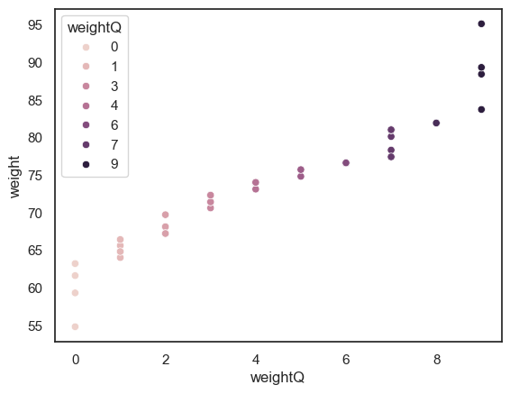
To visualise our new variable, we will use a scatterplot, where each data point shows an individuals weight and and the associated weightQ

sns.scatterplot(data = data, x = "weightQ",  y = "weight", hue = "weightQ")

<Axes: xlabel='weightQ', ylabel='weight'>