
4.5. Effect size (Pearson’s \(r\))#
For correlations, the effect size is given directly by the correlation coefficient, Pearson’s \(r\).
Recall that an effect size quantifies how large the effect of interest is relative to random variation.
In the case of a correlation, the effect of interest is the relationship between \(x\) and \(y\) described by the best-fitting line \(y = mx + c\), while the random variation is the scatter of data points around this line.
Pearson’s \(r\) captures exactly this balance between signal and noise. You may recognise this idea from the figure in the section on Correlation in the chapter Describing Data (it may be helpful to revisit it here).
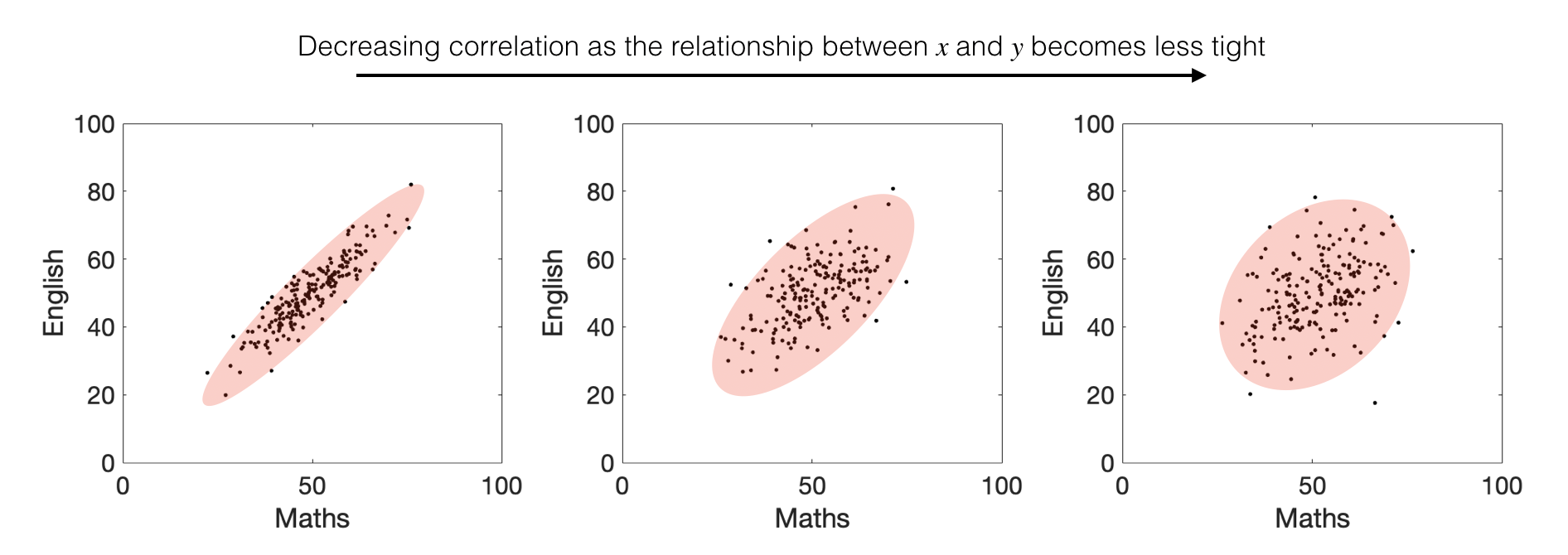
The correlation coefficient \(r\) always lies between 1 and −1. A value of \(r = 1\) indicates a perfect positive linear relationship (all points lie exactly on an increasing straight line), while \(r = -1\) indicates a perfect negative linear relationship.
Correlation therefore provides a pure measure of the strength of the relationship between \(x\) and \(y\), because it is standardised to account for the spread of values in \(x\) and \(y\) independently.
4.5.1. Effect size \(\neq\) statistical significance#
As with differences in means, whether a correlation is believable or statistically significant depends not only on its size, but also on the sample size \(n\).
Consider the examples below:
The correlations in the top row are all based on a small sample size (\(n = 12\)).
The correlations in the bottom row are based on a much larger sample size (\(n = 200\)).
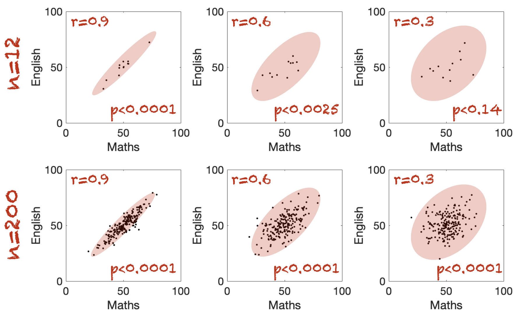
The red oval captures the overall shape of the cloud of points: a more elongated shape corresponds to a stronger correlation and a larger effect size.
However, for a given effect size, a correlation is less convincing when the sample size \(n\) is small. This increased uncertainty is reflected in the statistical significance, as shown by the corresponding \(p\)-values.
Statistical significance of \(r\)#
For a given values of Pearson’s \(r\), we can actually test the significance of the correlation using a one-sample \(t\)-test.
We calculate a \(t\)-score using the equation:
and then the \(p\)-value is obtained from the \(t_{n-2}\) distribution.
However you can get straight to the \(p\)-value by using scipy.stats - note that we are using scipy.stats as the other correlation functions we met in numpy and pandas do not return a \(p\)-value.
Here is the syntax to test the correlation between Maths and English scores, assuming these are columns in a dataframe scores:
stats.pearsonr(scores.maths, scores.english).pvalue
What counts as a large effect#
Wikipedia tells me that \(r\) values of 0.1, 0.3 and 0.5 are considered small, medium and large respectively
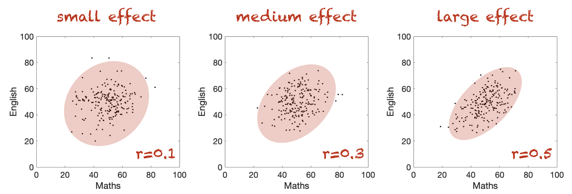
… but bear in mind this is just a rule of thumb.