3.8. Inference from a sample

The Central Limit Theorem tells us that, for large \(n\), the sampling distribution of the mean follows a Normal distribution: \(\mathcal{N}(\mu, \frac{\sigma}{\sqrt{n}})\).

If we know the parent distribution (as we did for the UK Brexdex distribution), then we also know the parameters \(\mu\) and \(\sigma\). This allows us to calculate the sampling distribution of the mean for samples of size \(n\), or to simulate it directly as we did previously. Some examples of known parent distributions include: standardized tests such as IQ tests or SATs, where the population mean and standard deviation are defined.

However, a more common situation in experimental science is that we only have data from our sample, not from the entire population. This means we usually don’t know the population parameters \(\mu\) and \(\sigma\)

Despite this, we often want to make inferences about the population based on the sample data. In particular, we want to estimate a plausible range in which the true population parameters \(\mu\) and \(\sigma\) might fall.

In this section we look at how we can do this.

3.8.1. Set up Python libraries

As usual, run the code cell below to import the relevant Python libraries

# Set-up Python libraries - you need to run this but you don't need to change it
import numpy as np
import matplotlib.pyplot as plt
import scipy.stats as stats
import pandas as pd
import seaborn as sns
sns.set_theme(style='white')
import statsmodels.api as sm
import statsmodels.formula.api as smf
import warnings 
warnings.simplefilter('ignore', category=FutureWarning)

3.8.2. Example sample

Let’s test our ability to make inferences from a sample. Suppose I hypothesise that students taking A-level maths have higher than average IQ scores. Because IQ tests are standardized, the population mean IQ score is 100.

To test this hypothesis I obtain a sample of IQ scores for 60 students taking A-level maths (note - these are made up data!):

mathsIQ_60 = pd.read_csv('https://raw.githubusercontent.com/jillxoreilly/StatsCourseBook/main/data/mathsIQ_60.csv')

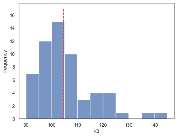
print('mean IQ = ' + str(mathsIQ_60.IQ.mean()))

mean IQ = 104.6

I can see that the mean IQ of the students in my sample is indeed slightly above 100. A quick look at the histogram with the mean marked in red suggests a positive skew, that is, some students have IQ well above the mean but none have an IQ well below the mean.

sns.histplot(mathsIQ_60.IQ, bins=range(90,150,5))
plt.plot([mathsIQ_60.IQ.mean(), mathsIQ_60.IQ.mean()], [0,17], 'r--')
plt.xlabel('IQ')
plt.ylabel('frequency')
plt.show()

3.8.3. From Sample to Inference

… but these data represent just a single sample of maths students - 60 students out of the thousands of possible!

Could the high mean IQ be due to random chance, as I happened to select a sample containing several high IQ students?

What I need to do is move from what I know about the sample of maths students to what I can infer about the population of maths students.

• Note that the population of maths students is not necessarily the same as the general population (whose mean IQ is known to be 100 because IQ is a standardized test).

Imagine I had measured the IQs of the whole population of maths students…

If i had truly measure the IQs of all maths studnets, then I could find the population parameters \(\mu\) and \(\sigma\) (e.g. using population.mean() and population.std()) as I did in the Brexdex examples, when we did have access to the parent distribution.

In that case, I would know the true mean of all maths student and with this knowledge could directly compare it to the general population mean (which is 100). Even a small difference of a single IQ point could then be considered meaningful, because we’d be comparing two entire popultions, not uncertain estimates based on samples.

If we did have access to the entire parent distribution, I could then draw many samples of size \(n\) from that population. As long as \(n\) was large enough, the Central Limit Theorem would tell us that the sampling distribution of the mean is a normal distribution $\( m \sim \mathcal{N}(\mu, \frac{\sigma^2}{\sqrt{n}}) \)$

But in reality…

We don’t acutally know what \(\mu\) or \(\sigma\) are. So instead we will explore how plausible different values of \(\mu\) would be, given our sample mean

• for now we are just going to assume that \(\sigma = s\).

Likelihood distribution of \(\mu\)

If we knew \(\mu\) and \(\sigma\) (note: we actually don’t) then we could work out the probability of getting the observed sample mean \(m=104.6\) as follows:

\[ m \sim \mathcal{N}(\mu, \frac{\sigma^2}{\sqrt{n}}) \]

so the probability of obtaining a sample mean of m (or higher) is

stats.norm.cdf(m,mu, sigma/n**0.5)

… Remember that in Python s/n**0.5 represents \(\frac{s}{\sqrt{n}}\), the (estimated) standard error of the mean.

Let’s assume (for now) that \(s\) (the sample standard deviation, mathsIQ_60.IQ.std()) is a good estimate of the population standard deviation.

• spoiler - this in fine for \(n>50\) when the central limit theorem applies

• later (in the section on the \(t\)-test) we will meet the \(t\) distribution which takes into account uncertainty about \(sigma\) when the sample size is small

Then the sampling distribution of the mean would be

\[ m \sim \mathcal{N}(\mu, \frac{s^2}{\sqrt{n}}) \]

Then for any proposed value of the population mean \(\mu\), we can work out the probability of obtaining \(m=104.6\) in a sample is given by the normal CDF. for example, what would be the probability of \(m=104.6\) if \(\mu=102.1\)?

stats.norm.cdf(104.6, 102.1, (s/n**0.5))

… noting that s/n**0.5 is Python for \(\frac{s}{\sqrt{n}}\), the (estimated) standard error of the mean.

Building the Liklihood Function

If we repeat this process for all possible values of \(\mu\), we end up with plot of how likely our sample mean would be if each possible value of \(\mu\) were true. This is called the likelihood function and it tells us how likely each possible value of \(\mu\) would be to produce our sample mean \(m\)

We can then take a leap and say:

• If I need to guess the true value of \(\mu\), my best guess is the one that was most likely to produce the observed sample mean \(m\)

• Then my best estimate of \(\mu\) is in fact \(m\)

• The likelihood that other values of \(\mu\) produced the sample mean \(m\) is quantified by the likelihood function.

Video

Here is a video explaining how we get the likelihood function by trying lots of different possible or ‘candidate’ values for the population mean \(\mu\), and imagining the sampling distribution of the mean that would arise:

%%HTML
<iframe width="560" height="315" src="https://www.youtube.com/embed/pQVaBpDaAgw?si=Kp3i6i2atH7ksdpK" title="YouTube video player" frameborder="0" allow="accelerometer; autoplay; clipboard-write; encrypted-media; gyroscope; picture-in-picture; web-share" referrerpolicy="strict-origin-when-cross-origin" allowfullscreen></iframe>

3.8.4. Plot the likelihood distribution

That last bit probably seemed a bit abstract. Luckily, we can easily plot the likelihood distribution. This will show us how plausible different values of the population mean \(\mu\) are, given our observed sample mean.

To do this, we first choose a range of possible values of \(\mu\) that we want to test:

mu = np.arange(95,115,0.1) 
# this is a list of 'candidate' values for the unknown population mean, mu

for each possible value of \(\mu\), work out the probability of the observed sample mean \(m\) if that value of \(\mu\) were true. This represents the likelihood of \(\mu\) given our observed sample mean \(m\))

Once we’ve calculated these likelihoods, across a range of possible values for \(\mu\) we can plot them!

m = mathsIQ_60.IQ.mean() # sample mean
s = mathsIQ_60.IQ.std() # sample s.d.
n = len(mathsIQ_60.IQ) # sample size
SEM = s/(n**0.5) # standard error of the mean

# calculate the probability of the observed sample mean n
# IMAGINING: IF each value of mu WERE TRUE
p = stats.norm.pdf(mu,m,SEM)

# plot the likelihood distribution for mu
plt.plot([m,m],[0,0.3],'r--')
plt.legend('m') # add the sample mean for comparison
plt.plot(mu,p,'k-')
plt.xlabel('possible values of $\mu$')
plt.ylabel('likelihood')

plt.show()

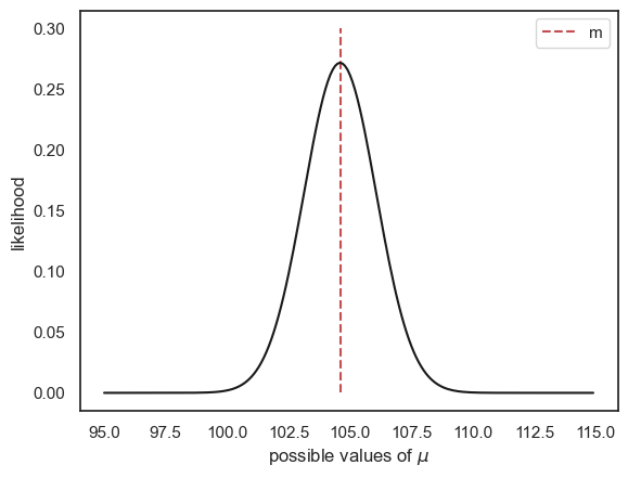
Ta-daa - this plot tells us how probable our observed sample mean would be given each possible value of \(\mu\) and conversely, how \(likely\) each true value of \(\mu\) is, given the observed data.

• Watch out! There is a real value of \(\mu\) and it is a single number, not a distribution

• You can think of the likelihood distribution as a belief distribution

  • By analogy, say I ask you to estimate the height of your statistics lecturer

  • Since you are uncertain, we could plot a graph of how likely you think each value is (unlikely that she is 150cm or 200cm tall, but a range of values, perhaps around 165cm, are considered likely)

  • This does not mean that the actual height of the statistics lecturer is a distribution! She is not taller some days and shorter on others! Her height is a fixed and exact number, it is just your belief about her height that is a distribution.

The liklihood distribution works the same way. It represents our uncertainty about \(\mu\), not variability in \(\mu\) itself