2.3. Rank-based tests

Here we review a class of statistical tests based on replacing data with their ranks.

We start by considering why this approach might be advantageous, given that we have already met another method (permutation testing) which is very powerful and is appropriate in most situations.

2.3.1. Permutation tests assume the population is similar to the sample

In general, if we draw a small sample of data from a larger population, the distribution of data within the sample resembles the distribution in the population.

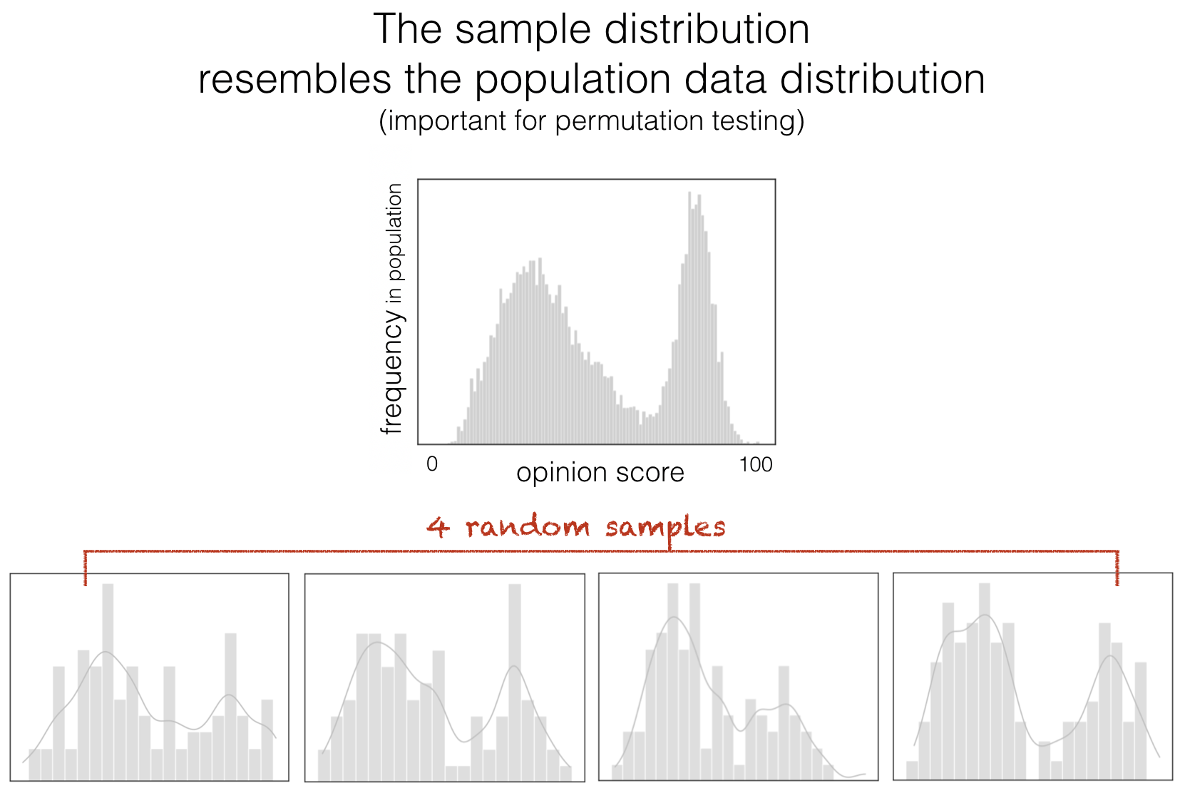
The figure above shows four random samples of 100 individuals drawn from the bimodal distribution above. These are made-up data, but you can think of them as something like scores out of 100 representing people’s opinions on a polarizing issue, such as how migrants should be treated or whether inheritance tax is fair. In this kind of situation, people tend to have either high scores or low scores, with relatively few holding a neutral opinion.

You will see that the data distribution within each sample resembles the original population (having two peaks).

Permutation testing, which we introduced in the previous section, makes use of the idea that the distribution of data in a (small) sample can be treated as representative of the population as a whole. Under the null hypothesis, group membership is assumed not to matter, so we shuffle the data while ignoring which group each observation originally belonged to. This shuffling process generates many “new” random datasets, allowing us to estimate how much the sample mean would vary from sample to sample purely due to chance—that is, because different datapoints happen to be included in each sample.

The exact distribution of the sample mean across the shuffled datasets (the null distribution) naturally depends on the data distribution itself. In this case, we are implicitly assuming that the distribution of the data we are shuffling (the sample) is representative of the population data distribution as a whole.

2.3.2. But small samples may not be representative

When we are working with a sample of data, especially a small sample, there is always a risk that the sample is not representative of the wider population.

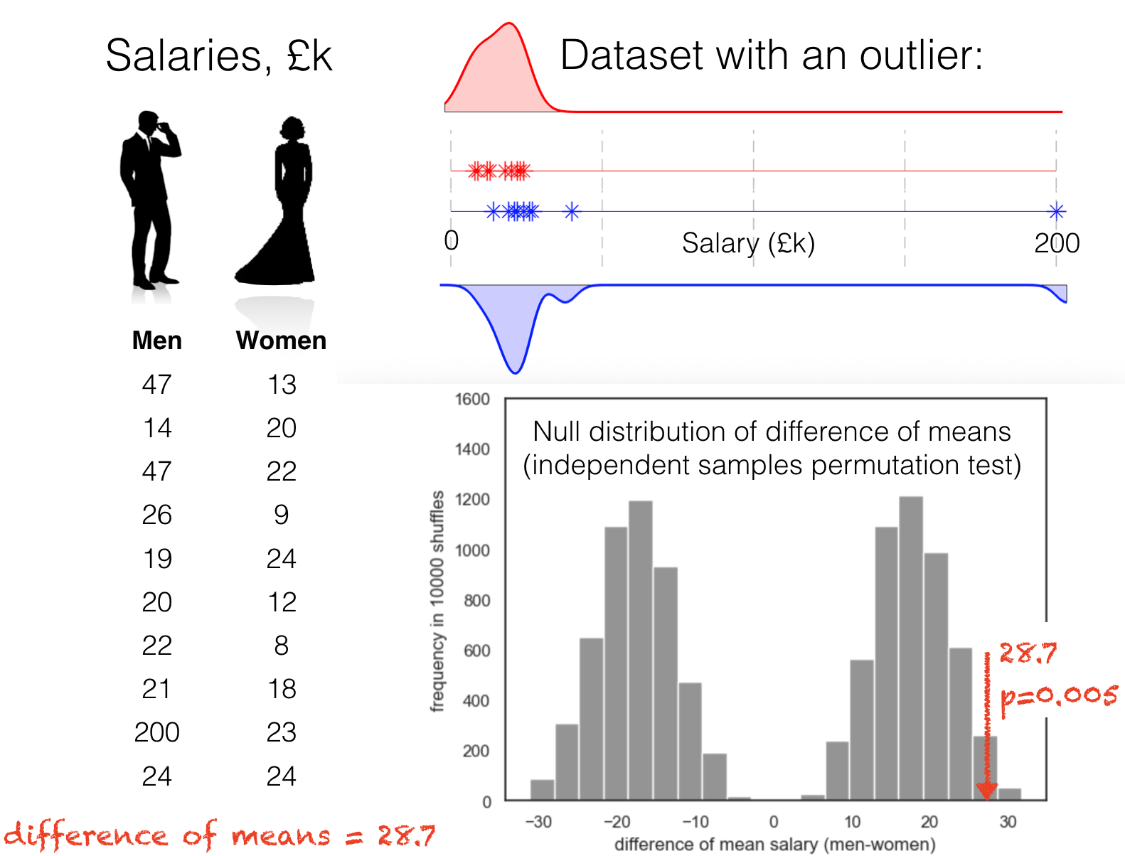
For example, consider these salary data for men and women. There happens to be a huge outlier in the ‘men’ group - someone who earns £200k, whilst everyone else earns less than £50k.

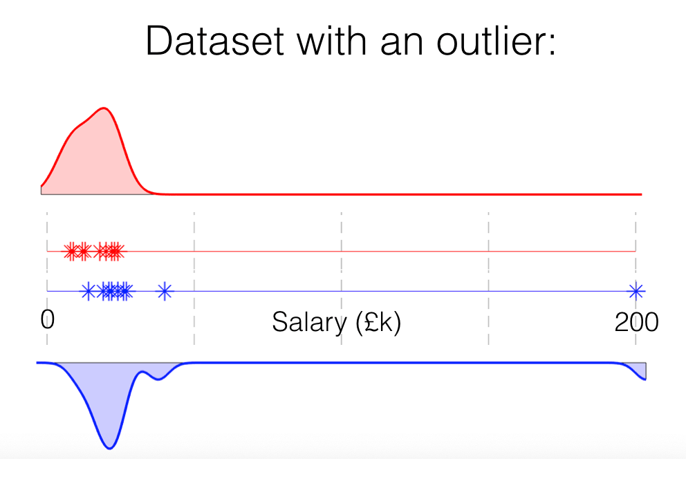
Because there are only 20 people in our sample, generalising from this sample to the population (which we implicitly do when running a permutation test) means accepting that 1 out of 20 people (5%) earn £200k, even though in reality the true proportion is much smaller (closer to 1%).

2.3.3. Outliers can have a big effect on our statistical tests

In permutation testing case, we shuffle up everyone’s salaries and assign the labels ‘man’ and ‘woman’ randomly. Then we ask how often we get a difference of means as large as the observed value (in this case £28k) in shuffled data - because such difference in shuffled data must be due to chance, this allows us to quantify how likely our observed value would be to arise due to chance.

If we do that we can see that the shuffled difference of means fall into two completely separate groups - cases where the £200k person was labelled as a man, and cases where they were labelled as a woman. Arguably, this means our conclusions depend pretty heavily on the single observation that one man had a very high salary.

Note, that such extreme outliers can arise by chance (for example, if we happen to sample someone who is atypical), but they can also result from measurement error (such as a noisy reading from a brain imaging machine) or from user error (for example, incorrect data entry), as discussed previously in the Data Wrangling section.

2.3.4. Replacing data with their ranks reduces the effects of outliers

One way to make an analysis less sensitive to outliers is to work with the ranks of the data rather than the raw data values themselves. When we rank data, the smallest value is assigned rank 1, the next smallest rank 2, and so on. The largest value then receives rank ( n ), where ( n ) is the sample size.

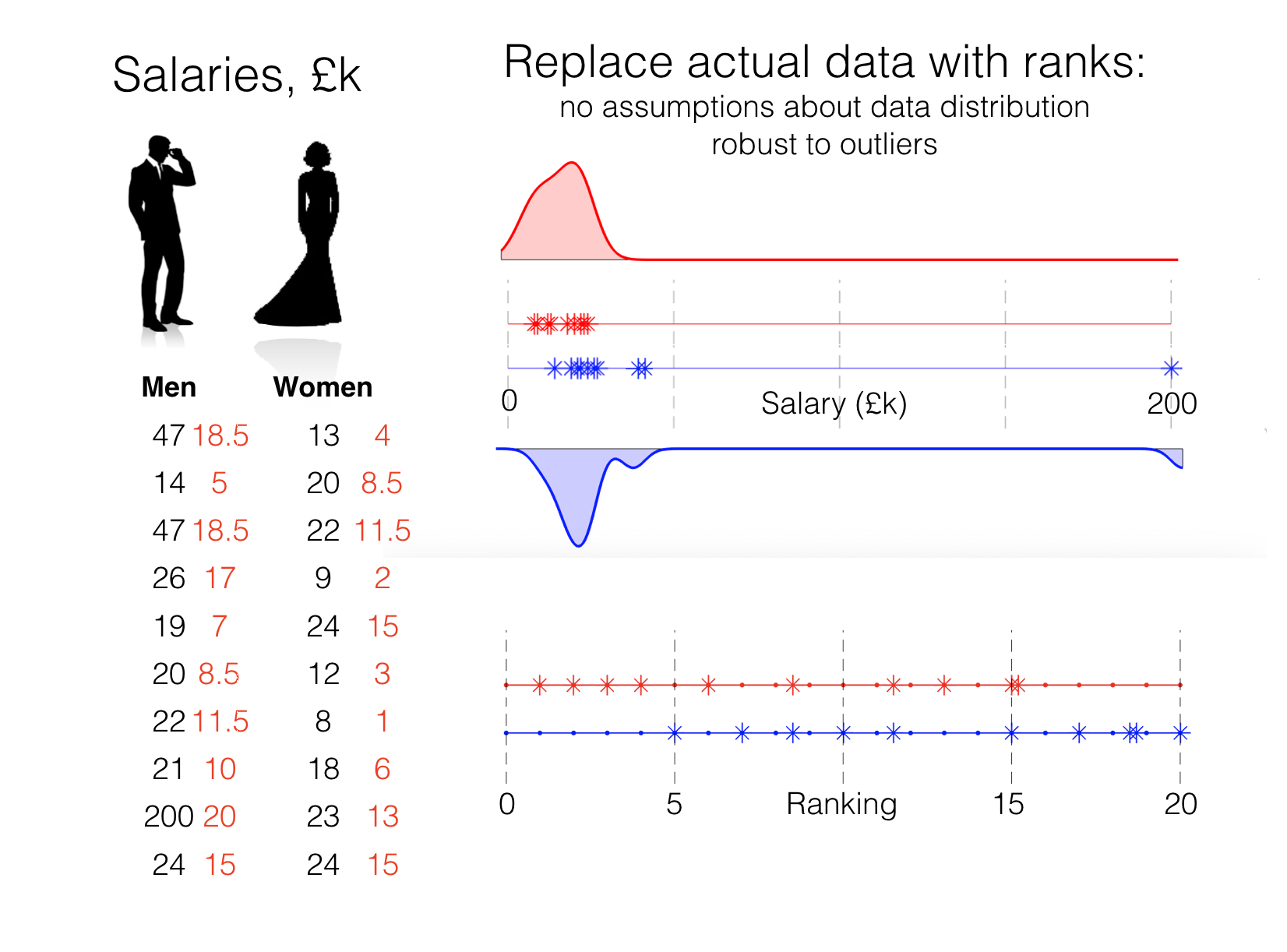
Because the largest value is always assigned rank ( n ), regardless of its numerical size, ranking the data substantially reduces the influence of outliers:

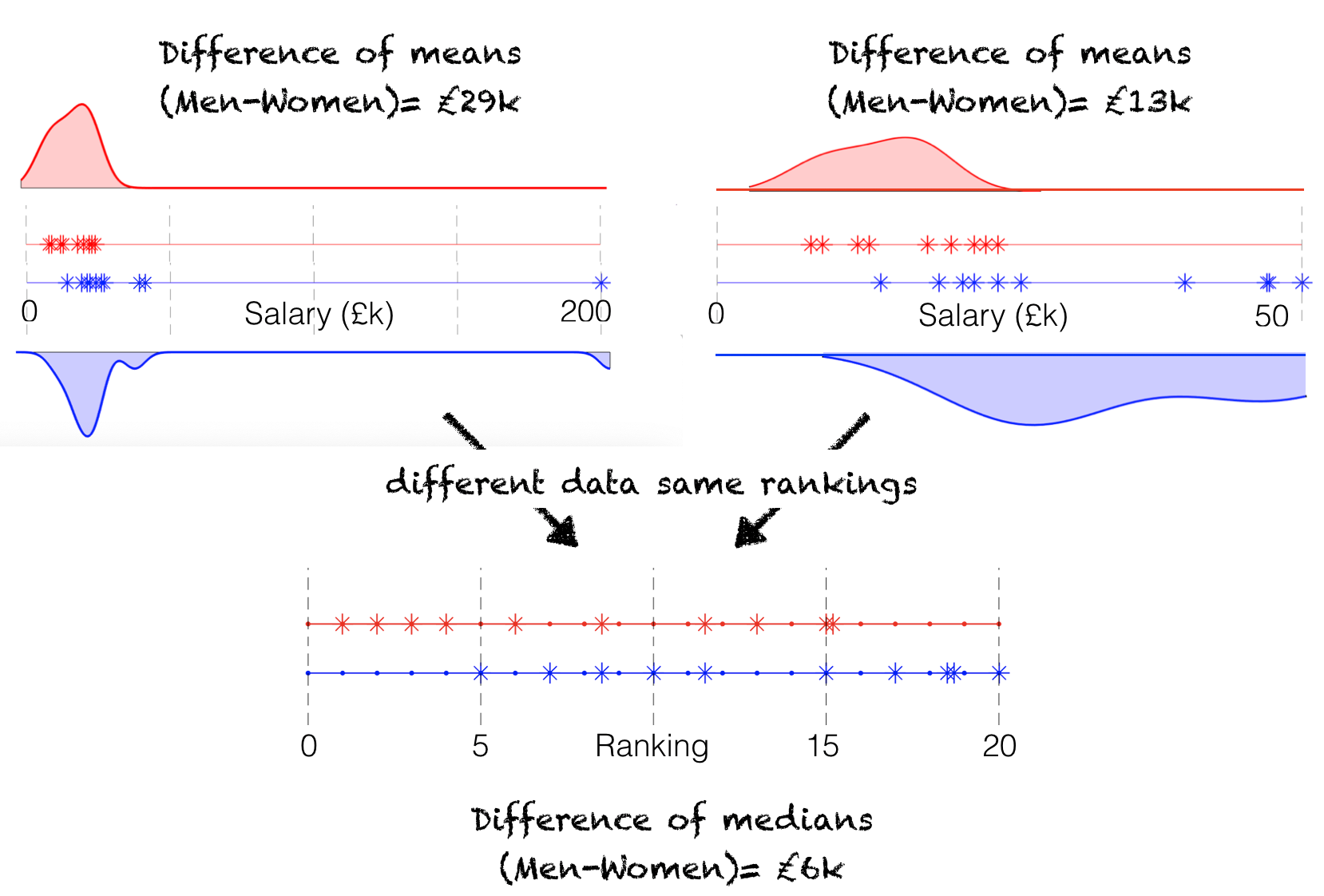
Having converted the data into ranks, we can then ask whether the proportion of high ranks falling into one category (and, correspondingly, the proportion of low ranks falling into the other category) is greater than we would expect by chance.

In the salary example, the four highest-ranked individuals in the dataset are men, because the four highest salaries all belong to men. More generally, a larger proportion of the higher ranks fall into the “men” group.

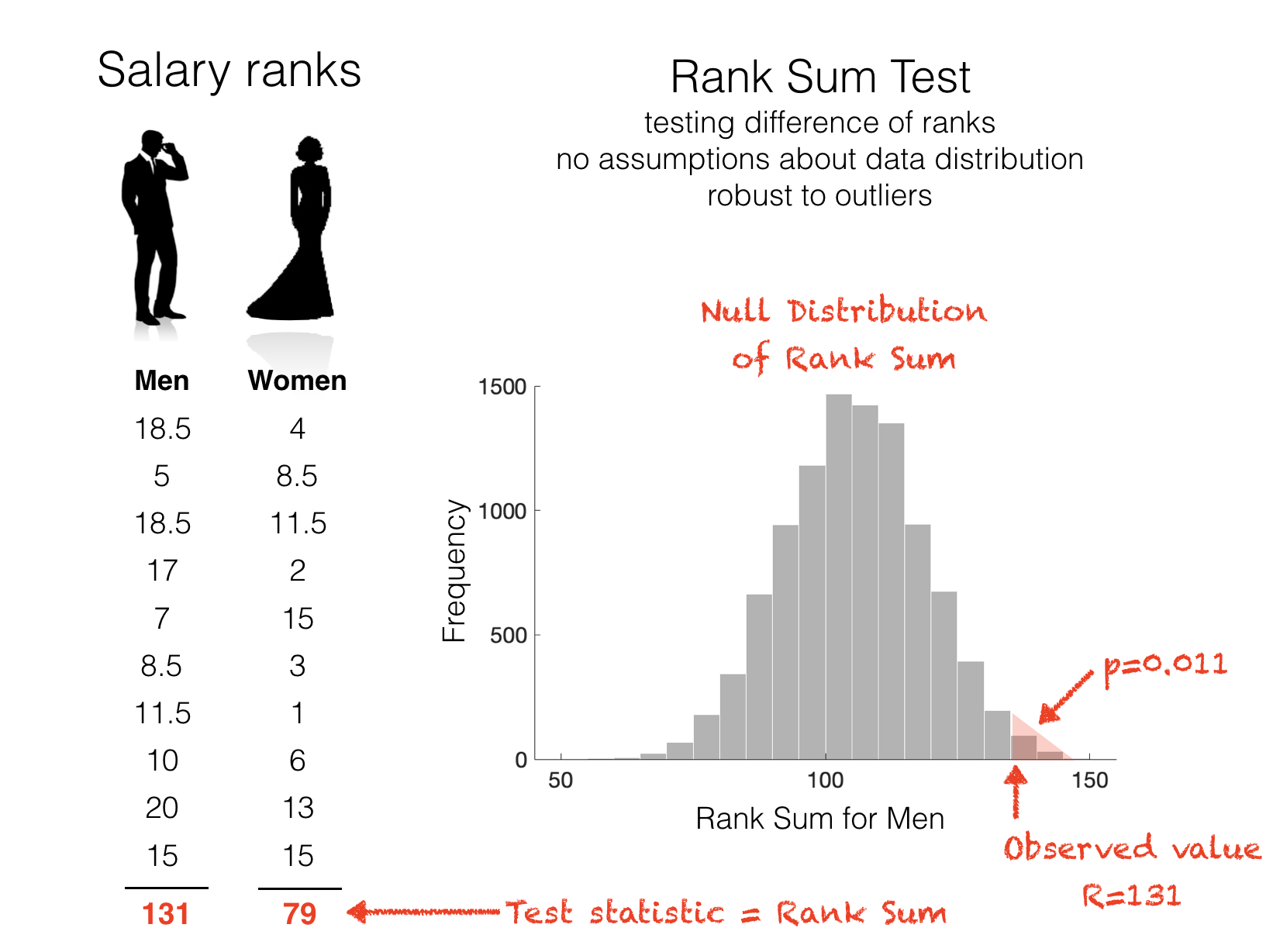
We summarise how many of the high ranks ended up in the “men” group using the rank sum (see the worked example on the next page). For our observed data, the rank sum is 131.

2.3.5. Null distribution of the Rank Sum

Under the null hypothesis, we would expect high and low ranks to be equally likely to fall into the “men” and “women” categories.

We can generate the null distribution of the rank sum by effectively permuting the ranks rather than the original data values.

• In fact, the null distribution of the rank sum can be derived exactly using a formula that considers all possible permutations of ranks, but we do not need to go into those details here.

2.3.6. Null distribution based on ranks is not so sensitive to the outlier

Compare the shape of the null distribution of the rank sum to that of the null distribution of the mean differece.

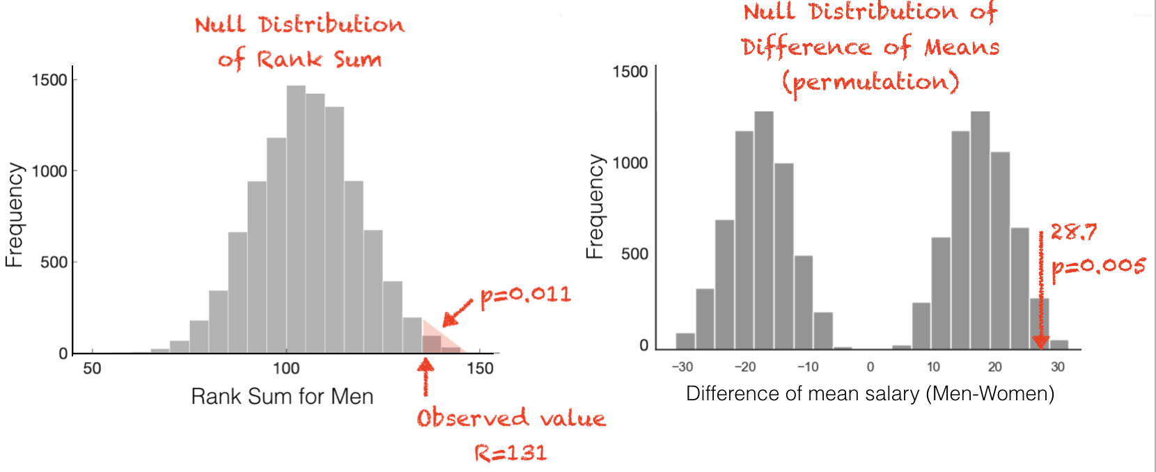
We can see that the influence of the extreme outlier is much reduced: the null distribution no longer shows two distinct peaks. As you may recall, those two peaks indicated that whether the difference in means favoured men or women depended strongly on whether the extreme outlier (the £200k individual) was labelled as a man or a woman.

2.3.7. Conclusions

A test based on ranks is more robust to outliers than a permutation test.

This is because the two approaches make different assumptions:

• The permutation test implicitly assumes that the sample data (including any outliers) are typical of the population.

• The rank-based test assumes only that the rankings of the data are typical of the population, which is a weaker assumption.