
3.9. Confidence intervals#
A 95% confidence interval is a range around a sample mean that reflects the uncertainty of our estimate.
Formally it is defined such that:
if we drew many independent samples (all of size n) from the parent distribution
… and we calculated an interval of that width around each sample mean
… then 95% of those intervals would contain the \(\mu\), the true mean of the parent population
Another way of thinking about it is:
For any one 95% confidence interval calculated from a single sample, we can be 95% confident that this interval contains \(\mu\), the true population mean.
So the confidence interval gives us a plausible range of values for the population mean, based on our sample data. As you will see our confidence interval will be subject to sample size and sample variability.
In this section we look at how we can construct confidence intervals.
3.9.1. Set up Python libraries#
As usual, run the code cell below to import the relevant Python libraries
# Set-up Python libraries - you need to run this but you don't need to change it
import numpy as np
import matplotlib.pyplot as plt
import scipy.stats as stats
import pandas as pd
import seaborn as sns
sns.set_theme(style='white')
import statsmodels.api as sm
import statsmodels.formula.api as smf
import warnings
warnings.simplefilter('ignore', category=FutureWarning)
3.9.2. Example sample#
Once again we use our sample of IQ scores for 60 students taking A-level maths (note - these are made up data!):
mathsIQ_60 = pd.read_csv('https://raw.githubusercontent.com/jillxoreilly/StatsCourseBook_2024/main/data/mathsIQ_60.csv')
Recall that:
the sample mean is 104.6 and
m = mathsIQ_60.IQ.mean()
print(m)
104.6
the sample standard deviation is 11.4
s = mathsIQ_60.IQ.std()
print(s)
11.366319559953567
3.9.3. Likelihood of a reference value#
Are A-level maths students smarter than average?
The mean IQ in the general population is 100.
We can ask: how probable the observed sample mean (\(m=104.6\)) would be if the sample of 60 maths students really came from a population with mean \(\mu=100\) (or lower) and standard deviation estimated as \(s\). Equivalently this tells us how likely it is that the true population mean for maths students is 100 or lower.
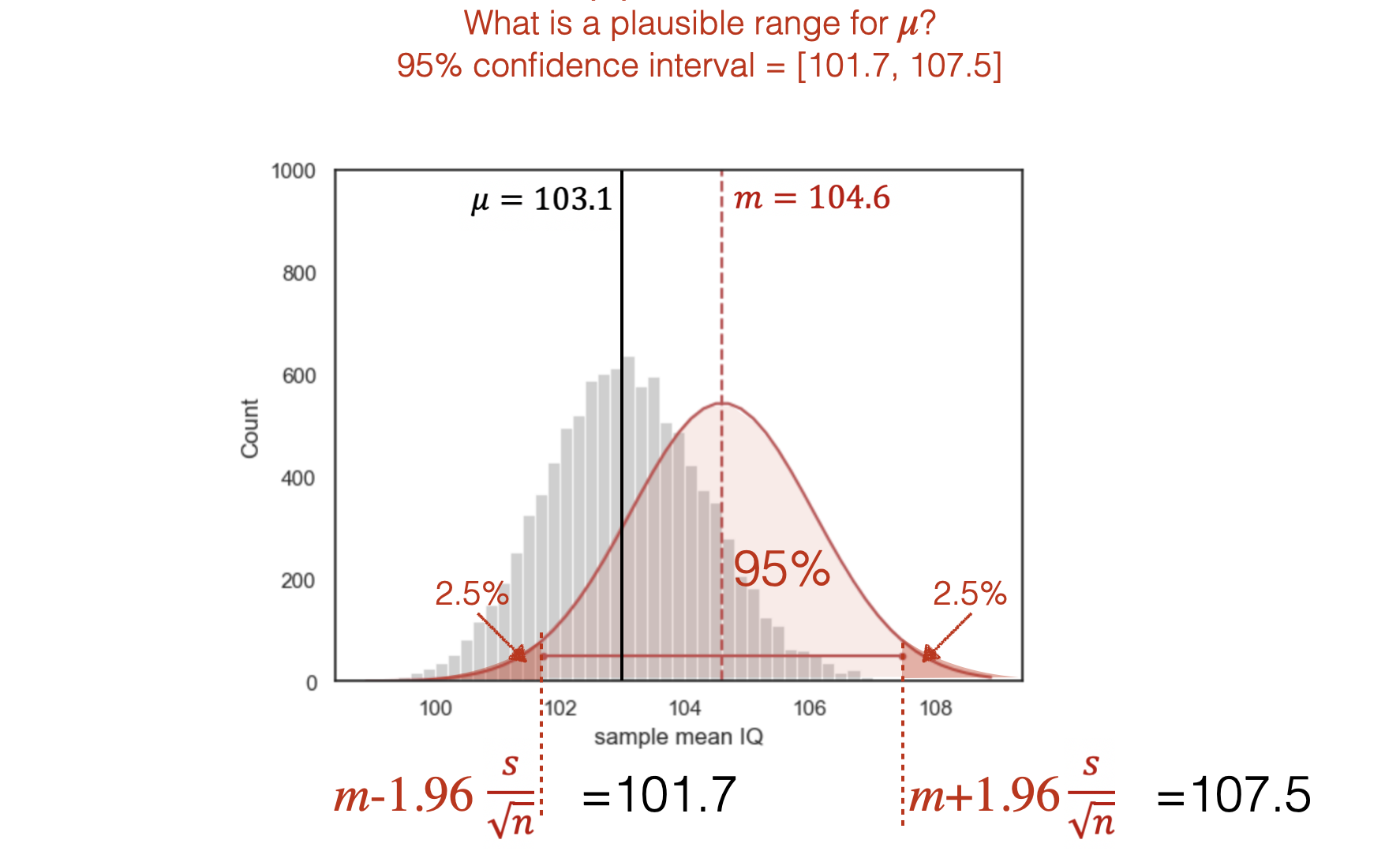
In our calculations we use the likelihood distribution that we calculated for the population mean \(\mu\) based on our sample:
\(\mu \sim \mathcal{N}(m, \frac{s}{\sqrt{n}}) \)
in this case:
\(\mu \sim \mathcal{N}(104.6, \frac{11.4}{\sqrt{60}}) \)
We can visualise this as :

In the plot:
the red curve shows the likelihood distribution for \(\mu\) based on our sample. Remember, this represents how plausible different population means are, given this observed data
The grey histogram shows the true sampling distribution of the mean for many samples drawn from the prarent population (for comparison)
Note, if we had used a different sample, with a different value of \(m\)<, we would get a different estimate of the probability that \(\mu \leq 100\)
Calculation with stats.norm.cdf()#
We can now calculate the exact probability that \(\mu \leq 100\) using stats.norm.cdf():
n=60
SEM = s/(n**0.5)
# percentage of time sample mean is expected to be less than 100 =

print(stats.norm.cdf(100,m,SEM)*100)
0.08597770891100479
Apparently, the likelihood that the population mean IQ for A-level maths students is 100, is quite low: 0.085%
Note, When we ask whether maths students are smarter than average, we’re really thinking about the probability of obtaining our observed sample mean if the true population mean were equal to or below the general population average (\(\mu \leq 100\)) There is a useful analogy here with the Blindsight example in the previous session:
In that case, we would conclude our patient was guessing if his performance was equal to or better than some criterion value which would rarely occur by chance.
In the same way, we conclude that maths student probably due obtain higher IQ score if their sample mean IQ is so high that it would be very unlikely to occur by chance under that alternative assumption that their true mean is 100 (or lower)
Check: Simulating from the population#
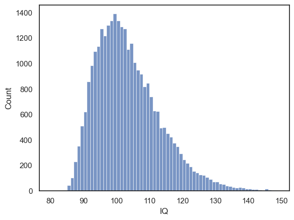
Just for fun, here is a much larger (made up) sample of all the students taking maths A-level (30,000 individuals)
Can you run a simulation to draw samples of size 60 from this dataset, get the mean of each one, and work out what percentage of sample means are indeed below 100?
Hopefully it should match fairly well the prediction from the Central Limit Theorem!
mathsIQ_30k = pd.read_csv('https://raw.githubusercontent.com/jillxoreilly/StatsCourseBook/main/data/mathsIQ_30k.csv')
sns.histplot(mathsIQ_30k.IQ, bins=range(80,150))
plt.xlabel('IQ')
plt.show()
# Your code here to draw 10,000 samples of size 60 from the distribution above
# Obtain the sample mean from each sample
# Work out the proportion of sample means that are less than 100

nReps=10000
m=np.empty(nReps)
samplesize=60

for i in range(nReps):
    sample = mathsIQ_30k.sample(n=samplesize,replace=False)
    m[i]=sample.IQ.mean()

print('The Proportion of sample means < 100 : ', str(sum(m<100)/len(m)))

sns.histplot(m)
plt.xlabel('IQ')
plt.title('Sample means from parent distribution')
plt.show()
The Proportion of sample means < 100 : 0.0045
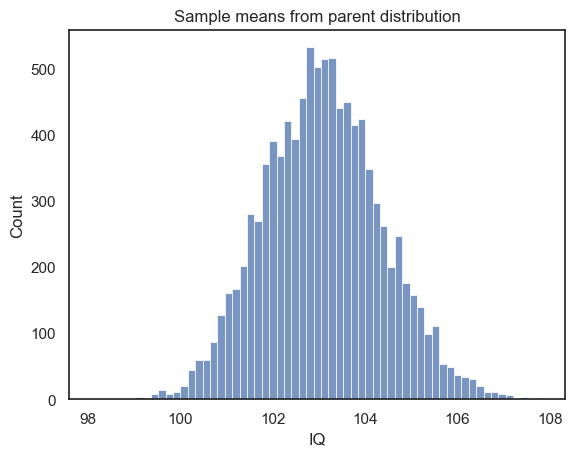
Hopefully the proportion of simulated sample means that are lower than 100 matches the prediction from the Central Limit Theorem - does it?
3.9.4. Confidence intervals#
The 95% confidence interval is the interval of the likelihood distribution that contains 95% of the area under the curve:
Therefore, a 95% confidence interval is an interval around a sample mean with a width such that for a single 95% confidence interval computed on a single sample, we (the researcher) have 95% confidence that that interval contains \(\mu\), the true mean of the parent population
Another way of thinking about this is that:
if we drew many independent samples (all of size n) from the parent distribution
… and we drew an interval of that width around each sample mean
… then 95% of those intervals would contain the \(\mu\), the true mean of the parent population
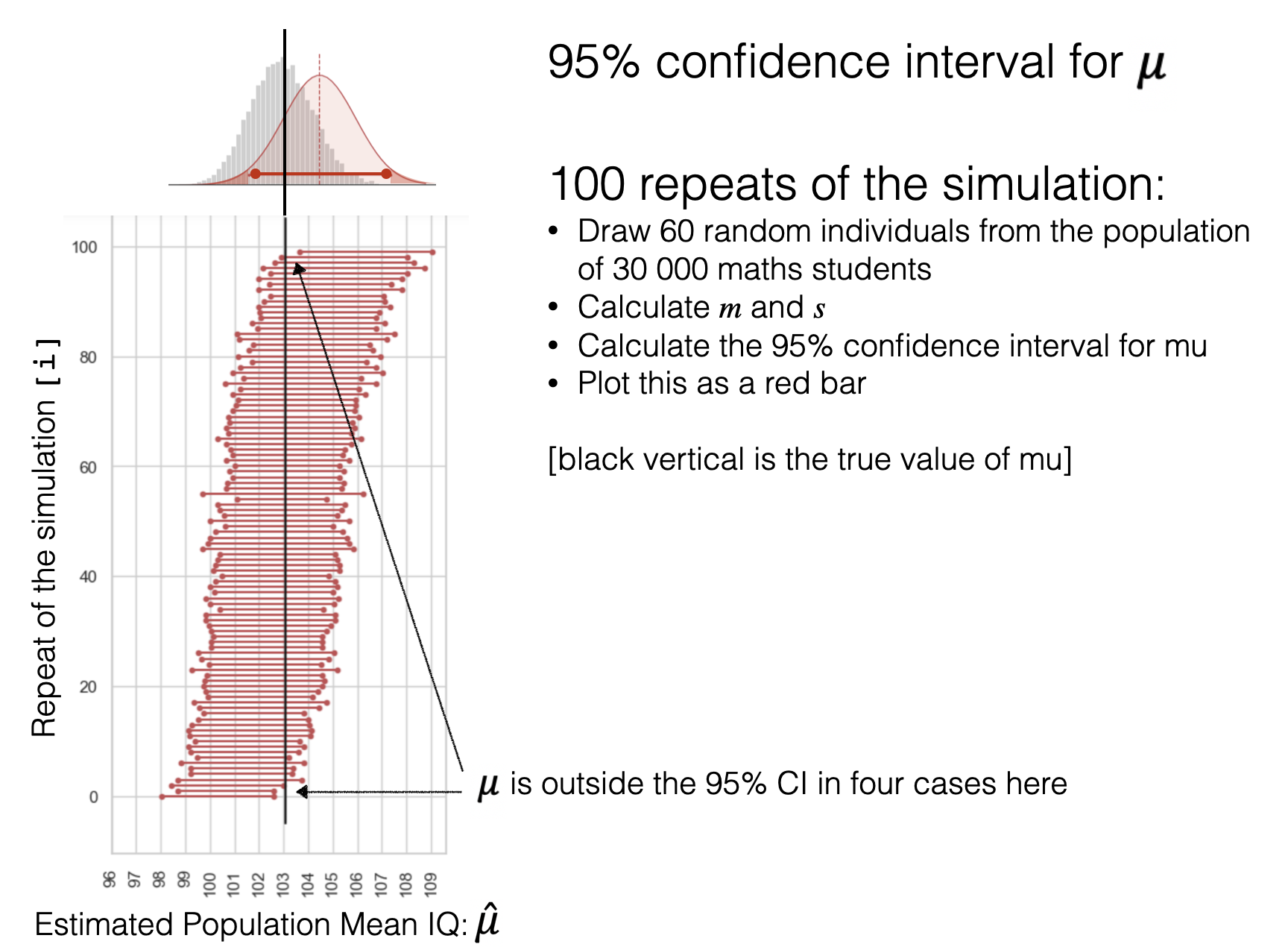
In the diagram below, I actually drew 100 samples of size 60 from my parent distribution (30,000 ‘maths students’) and calculated the 95% confidence interval for \(\mu\) from each sample, using the sample mean \(m\) and sample deviation \(s\).
note that \(m\) and \(s\) are different in each of the 100 samples

You can see that the position and width of the 95% CIs varies from sample to sample
However, if I put the samples in order (from lowest sample mean to highest) you can see that indeed, the 95% CI does contain the true population mean \(\mu\) in about 95/100 cases - actually 96/100 as this is ia random simulation
just a reminder that the population mean \(\mu\) is the mean IQ of A-level maths students, not the general-population mean of 100)
The magical \(Z=1.96\)#
For a normally distributed variable:
95% of cases fall within 1.96 standard deviations of the mean
99% of cases fall within 2.33 standard deviations of the mean
For example, say women’s heights in the UK follow a normal distribution \(\mathcal{N}(164.3, 6.1)\)
We expect 95% of women to have a height between \(164.3 - 1.96 \times (6.1)\), and \(164.3 + 1.96 \times (6.1)\), ie between 152.3 cm and 176.3 cm
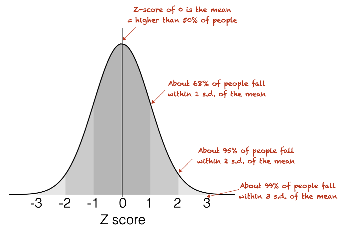
Remember the rule of thumb for the normal distribution:
95% CI for maths IQ#
The sampling distribution of the mean for the maths IQ data, with samples of size 60, was estimated to be \(\mathcal{N}(m, \frac{s}{\sqrt{n}})\) = \(\mathcal{N}(104.6, 1.47)\).
Our 95% CI for the mean of the parent population (mean IQ of all maths A-level students) is then
ie
That is, we are 95% confident that the true population mean IQ lies between 101.7 and 107.5.
Note that the mean of the general population (IQ=100) lies outside the 95% CI.