
3.4. The t distribution#
The \(t\) distribution describes the shape of the best-estimate sampling distribution of the mean when data are drawn from a normal distribution and the best-fitting normal distribution (ie, its mean and standard deviation) have been estimated from a small sample.
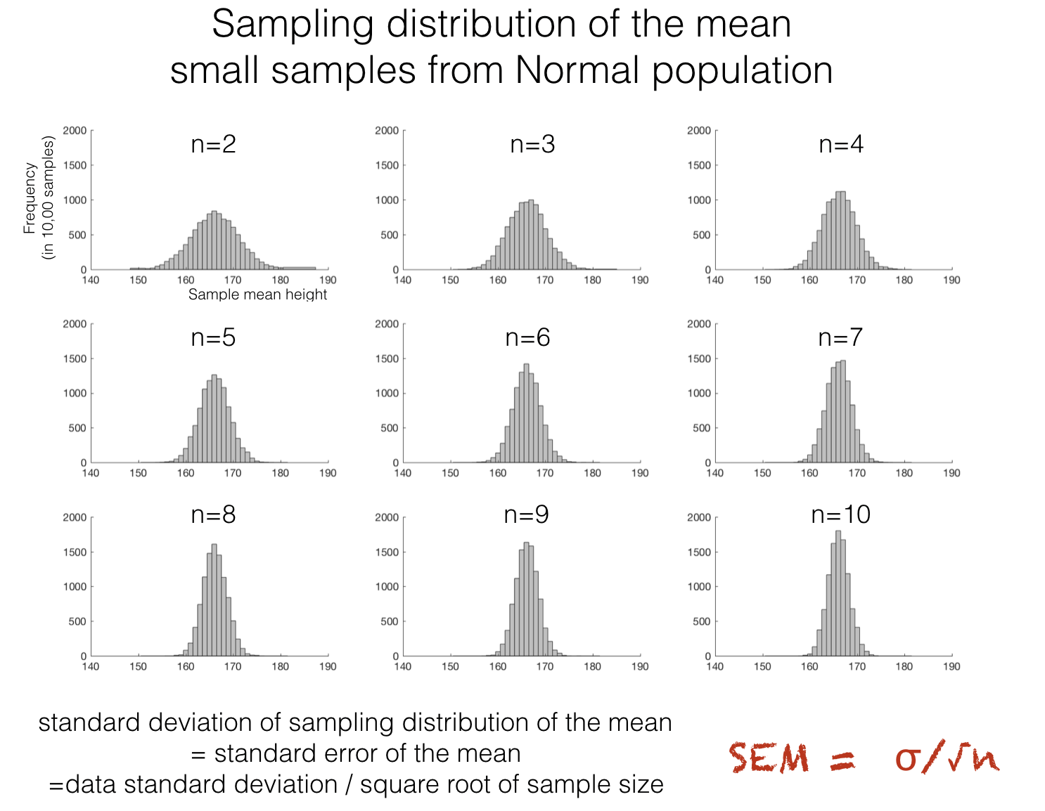
3.4.1. Sampling distribution of the mean#
The sampling distribution of the mean is the distribution you wuld obtain if you repeatedly took many different samples of size \(n\) from the population and calculated the mean for each sample
The null distribution is the sampling distribution of the mean (or different test statistic) that we would expect to observe if the null hypothesis were true
3.4.2. Scaling by sample size#
Recall from the previous lecture that the spread of the sampling distribution of the mean depends on the sample size. More precisely:
The standard deviation of the sampling distribution of the mean is the standard error, \(s/\sqrt{n}\) where \(s\) is the sample standard deviation and \(n\) is the sample size
3.4.3. Pointy top, heavy tails#
The \(t\) distribution looks a lot like the normal distribution, but it has a pointy top and heavy tails.
Importantly, the shape of the \(t\) distribution depends on the sample size used to estimate the best-fitting Normal distribution:
when the sample is tiny (\(n=2\)) we get an extreme pointy top and heavy tails
as the sample size gets large (about 30) the t distribution is almost identical to the normal distribution
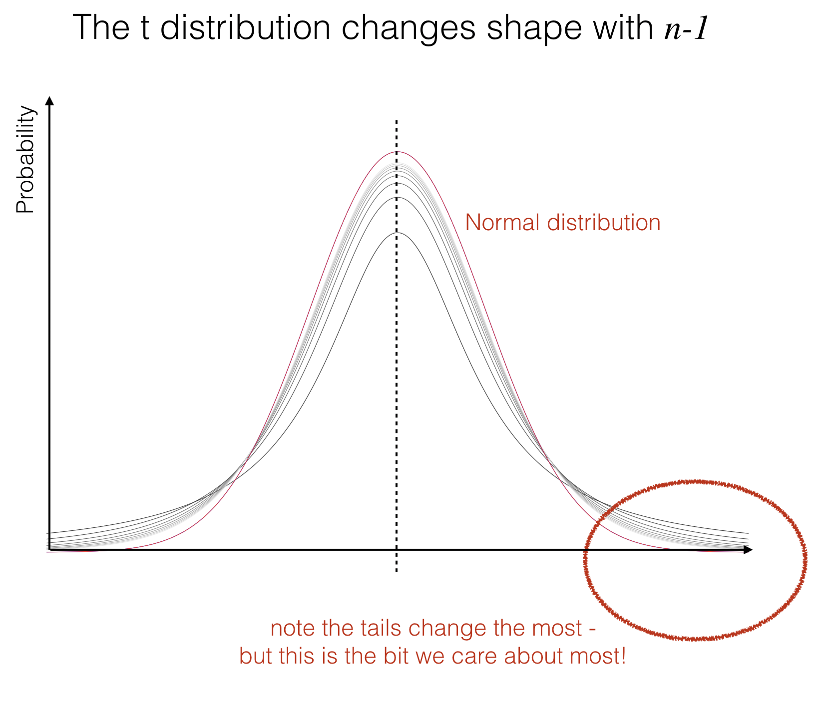
This distinction may seem subtle, but remember that a statistically significant result lies in the tails of the null distribution. If the \(t\) distribution represents the sampling distribution of the mean under the null hypothesis, then it is the behaviour of its tails that matters most.
In practice, we examine these tails to determine how likely it is that our observed result (such as a difference in means) could have arisen purely by chance.
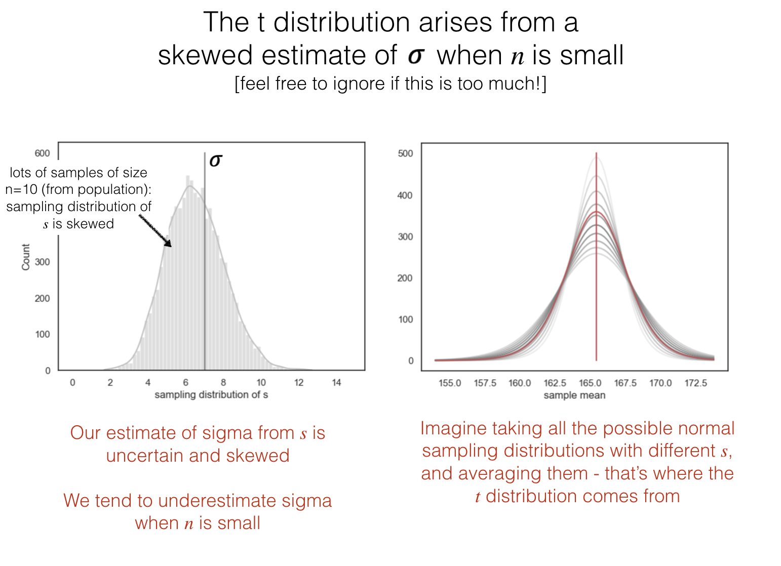
Why heavy tails?#
You can skip this bit if you don’t fancy it; it is sufficient to understand that the \(t\)-distribution has heavy tails because of ‘something to do with estimating the standard deviation’!
3.4.4. Analogy: \(t\) and \(Z\)#
We saw earlier that, if data are Normally distributed, then standardising the data by converting values to Z-scores produces a distribution with a fixed mean (0) and standard deviation (1).
If the data have sample mean \(\bar{x}\) and sample standard deviation \(s\), then each observation can be converted to a Z-score by:
From this standardised distribution, we can directly read off the probability of observing a given data value. For example, the probability of obtaining a Z-score greater than 1 is about 15%.
Similarly, for sample means, we can standardise them by converting them to \(t\)-scores:
This standardised distribution tells us the probability of obtaining a sample mean as large as our observed value \(\bar{x}\) (or larger) if the population mean were truly zero
This probability represents the chance of observing such a sample mean purely due to random sampling variation under the null hypothesis, when the null hypothesis states that the population mean is zero.
3.4.5. Link to t-test#
Of course, we don’t always expect our population mean to be zero under the null hypothesis. In the following sections, we see three examples
Single sample t-test#
Under the null, \((\bar{x}-\mu) = 0\), where \(\mu\) is a reference value and \(\bar{x}\) is the sample mean.
For example we hypothesise that Oxford students’ IQs are higher than the average (by definition the average IQ is 100)
\(\mathcal{H_o}\): Oxford students’ mean IQ is 100 \(\mathcal{H_a}\): Oxford students’ mean IQ is greater than 100
Then our equation to get the standardied \(t\) becomes:
Paired samples t-test#
Under the null, \((\bar{x-y}) = 0\), where \(x\) and \(y\) are paired values such as brothers’ and sisters’ heights, and \((\bar{x-y})\) is the mean difference in height between a brother and his own sister.
For example we hypothesise that men are taller than women:
\(\mathcal{H_o}\): The mean brother-sister difference is 0 \(\mathcal{H_a}\): The mean brother-sister difference is greater than 0
Then our equation to get the standardied \(t\) becomes:
Independent samples t-test#
Under the null, \((\bar{x}-\bar{y}) = 0\), where \(x\) and \(y\) are independent samples, and \(\bar{x}\) and \(\bar{y}\) are the means of those independent samples.
For example we hypothesise that Oxford students’ IQs (\(x\)) are higher than Cambridge students IQs (\(y\))
\(\mathcal{H_o}\): Difference of means is zero \(\mathcal{H_a}\): Difference of means (Oxford-Cambridge) is greater than zero
Then our equation to get the standardized \(t\) becomes:
… noting that \(s\) is now a combined standard deviation measure based on both samples, sommetimes called the ‘pooled variance estimate’; you don’t need t worry about how to calculate this as it is done automatically when you run the independent samples \(t\)-test in scipy.stats.