3.3. Best fitting Normal#
If we have some data \(x\), and we believe they come from a Normal distribution, we can describe the normal distribution they most likely came from as \(x \sim \mathcal{N}(m, s)\) where \(m\) and \(s\) are the mean and standard deviation we calculated from the data.
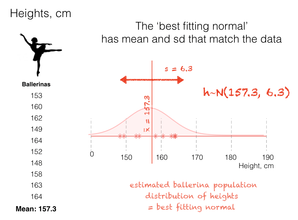
For example, given the heights of 10 fictional ballerinas, we can calculate the sample mean (157.3cm) and sd (6.3cm).
Using these two values, we can construct an estimate of the height distribution for all the ballerinas in the world (!) by assuming a Normal distribution with the same mean and standard deviation. This distribution is often referred to as the best fitting normal
3.3.1. By fitting the Normal we gain some information#
If it is reasonable to assume that heights are Normally distributed, then fitting the best-fitting Normal to our data gives us a fairly precise model of the heights of ballerinas worldwide. Importantly, this model should be more accurate than simply assuming that the population has exactly the same distribution as our sample, which may deviate from Normality due to sampling variability.
Compare the best fitting normals to the data KDE for ballerinas:
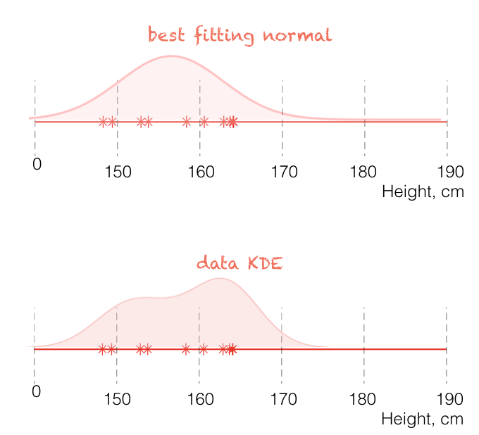
If heights in the population of ballerinas are indeed Normally distributed, then the best-fitting Normal provides a better estimate of the population height distribution. In this case, the apparent double peak in the KDE is best interpreted as a quirk of the small sample size (only 10 ballerinas), rather than a real feature of the population.
3.3.2. Incorrect assumption of normality#
If the data are not actually drawn from a Normal distribution, then the best-fitting Normal will be a poor estimate of the population data distribution.
In practice, non-Normal data distributions often contain outliers that would be extremely unlikely under a Normal model. When we try to fit a Normal distribution to such data, the fitted distribution is forced to be very wide in order to accommodate these outliers, resulting in a model that does not accurately represent the bulk of the data.
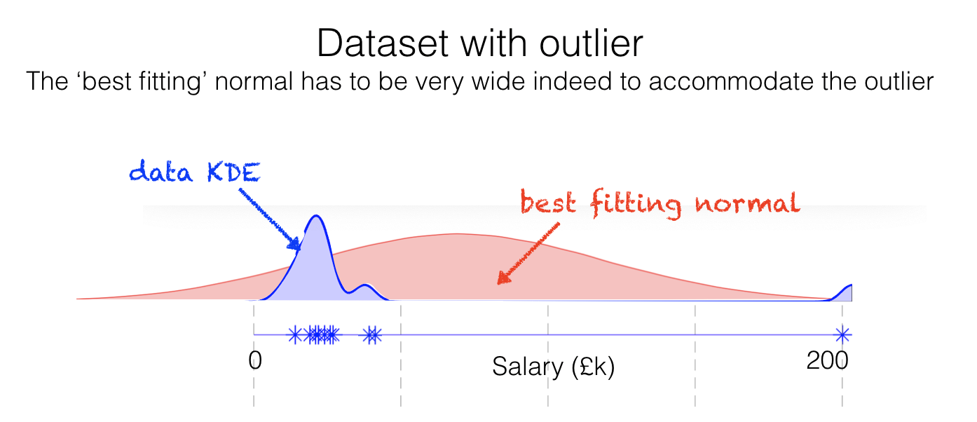
In the salary example shown above, the best-fitting Normal suggests that the most common salary is around £80k and that many people earn negative amounts of money. In this case, the population data is much more likely to be skewed - with a long positive tail - because of the natural boundary at zero. Here the best-fitting Normal is clearly neither a good match to the sample data nor a plausible estimate of salaries in the population as a whole.
3.3.3. The best fitting normmal is just an estimate#
The best-fitting Normal is a Normal distribution whose mean and standard deviation, (m) and (s), are calculated from the data.
Of course, even if the data are drawn from a truly Normal population, the sample mean and standard deviation from a small sample will not usually be exactly equal to the population mean and standard deviation. This is because samples are random: for example, we might happen to sample more particularly tall or particularly short ballerinas than we would expect on average.
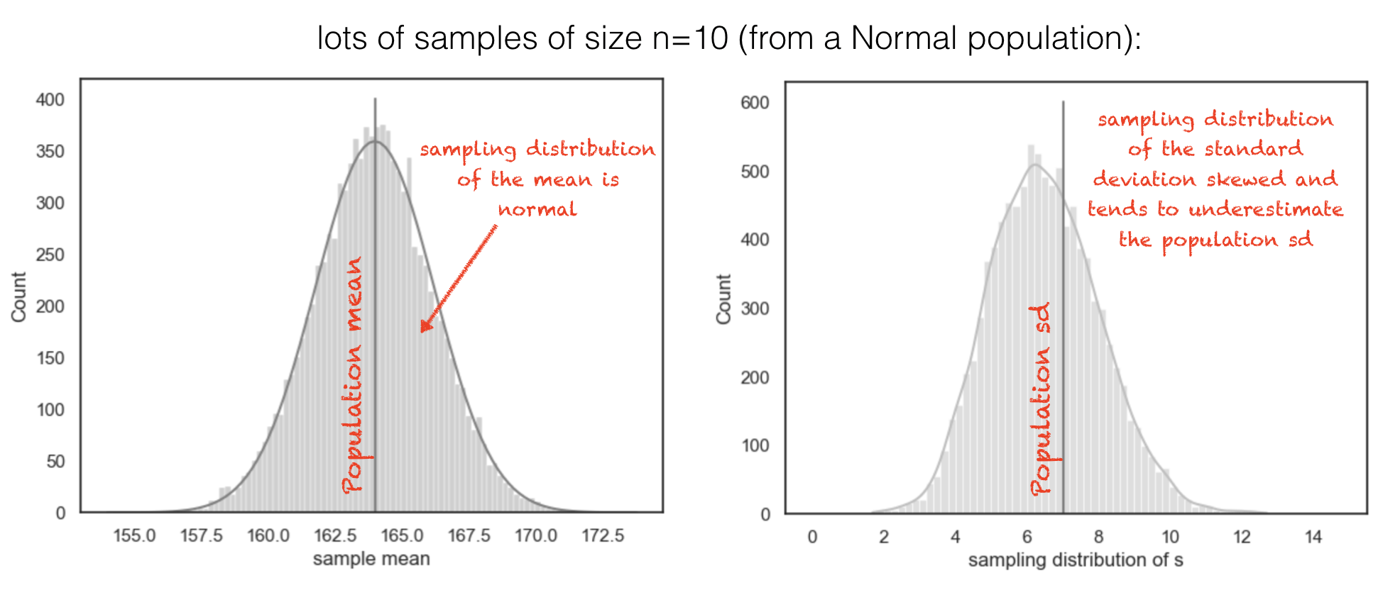
Below, I drew 10,000 samples of size (\(n = 10\)) from a large population of Normally distributed values, and calculated the mean and standard deviation for each sample:
Sample means are Normally distributed and centred on the true population mean.
Sample standard deviations have a skewed distribution and tend to underestimate the true population standard deviation.
Most importantly:
The sample mean and standard deviation are only estimates of the population mean and standard deviation, and they vary randomly from sample to sample.