
4.3. False positives and False negatives#
Here is a video about False Positives and False Negatives:
We can think of the hypothesis-testing framework as a 2×2 grid, contrasting reality (what is actually true) with our conclusions (what we decide based on the data and statistical test).
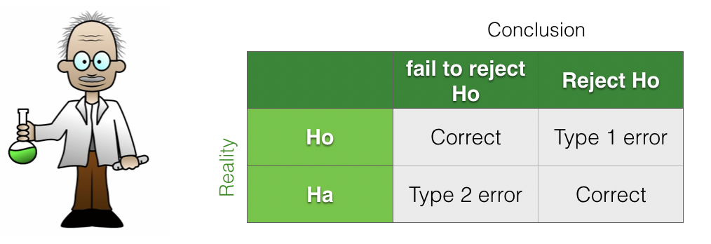
Within this framework, there are two ways to make an error:
We reject the null hypothesis when it is actually true (a Type I error, or false positive).
We fail to reject the null hypothesis when the alternative hypothesis is actually true (a Type II error, or false negative).
Because the terms Type I error and Type II error are easy to mix up, it is often clearer to use the terms false positive and false negative instead.
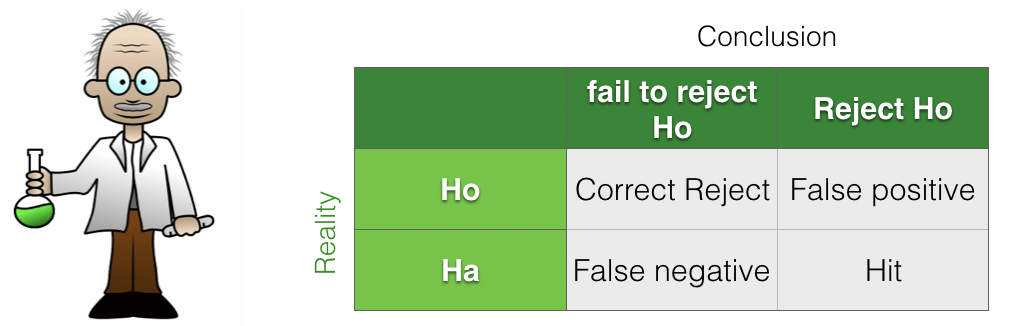
We can also describe the cases in which our conclusions are correct:
Hits: the alternative hypothesis \(\mathcal{H}_a\) is true, and we correctly detect this by rejecting the null hypothesis.
Correct rejects: the null hypothesis \(\mathcal{H}_0\) is true, and we correctly fail to reject it (slightly confusingly, a correct reject corresponds to correctly not rejecting the null).
4.3.1. Assuming \(\mathcal{H}_0\) vs assuming \(\mathcal{H}_a\)#
When we calculate a \(p\)-value for a statistical test, we assume that the null hypothesis \(\mathcal{H}_0\) is true and then ask how likely it is that we would obtain a result as extreme as the one observed purely by chance. In other words, we are reasoning under a specific assumed state of reality: that \(\mathcal{H}_0\) is true.
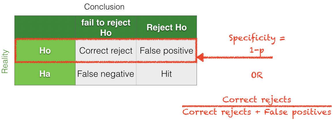
Assuming \(\mathcal{H}_0\) is true:
The \(p\)-value is the probability of making a false positive (rejecting \(\mathcal{H}_0\) when it is actually true).
Specificity is \(1 - p\), the probability of correctly not rejecting \(\mathcal{H}_0\) when it is true.
In contrast, in power analysis we consider the alternative state of reality in which the alternative hypothesis \(\mathcal{H}_a\) is true. Power is then the probability that we correctly reject the null hypothesis under this assumption.
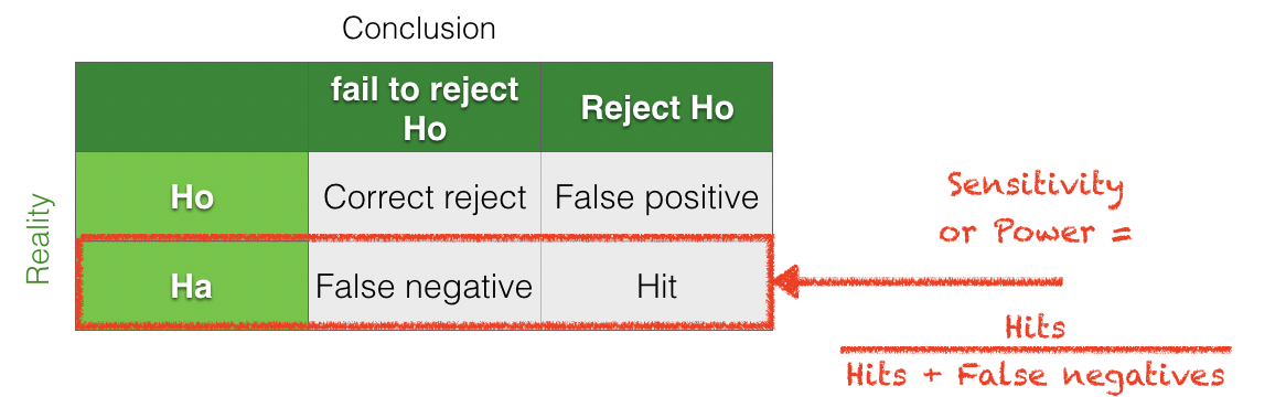
Assuming \(\mathcal{H}_a\) is true:
Power is \(1 -\) (the probability of a false negative).
Sensitivity is equal to power, that is, the probability of correctly detecting an effect when one truly exists.
Terminology
Because the terms sensitivity and specificity are easy to mix up, I prefer to focus on:
the \(p\)-value of a test (which corresponds to \(1 -\) specificity), and
the power of a test (which is equivalent to sensitivity).
4.3.2. Criminal analogy#
It can be helpful to think about hypothesis testing using an analogy to a criminal court:
\(\mathcal{H_o}\): Everyone is innocent until proven guilty
\(\mathcal{H_a}\): He’s guilty, dammit!
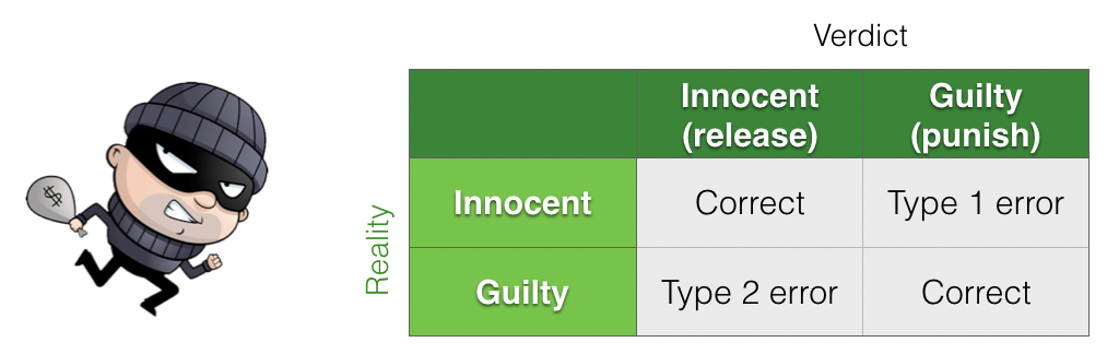
In this analogy:
A Type I error (false positive) is a wrongful conviction
A Type II error (false negative) is when the criminal gets away due to insufficient evidence
4.3.3. Trade-off#
There is always a trade-off between controlling the rates of false positives and false negatives. This is because, as scientists, we set the criterion for statistical significance.
If we set a very stringent criterion for significance, we reduce the chance of false positives, but at the cost of increasing the chance of false negatives. Conversely, using a more lenient criterion reduces false negatives but increases false positives.
Here is a video reviewing this idea:
4.3.4. Insufficient evidence#
The criminal analogy highlights the main cause of False Negatives (Type II errors) in scientific studies: insufficient evidence.Often if we fail to find a significant result, when there actually is an underlying effect, it is because the sample size is too small, therefore we don’t have sufficient evidence. This is because tests of statistical significance, and tests of statistical power, depend on three ingredients
The effect size
The sample size (\(n\))
The \(\alpha\) value (the cut-off \(p\)-value for significance)
In general,
The smaller the effect size, the larger the sample size neeed to detect it.
The more stringent the \(\alpha\) value, the larger the sample needed to detect an effect of a given size
\(\alpha=0.001\) is more stringent than \(\alpha=0.01\) etc
The next pages will cover the definition of effect size.
4.3.5. Sample size primarily affects power, not \(p\)-value#
Most people will accept the intuition that increasing the sample size should make an experiment ‘better’, more reliable or more believable. However it is worth understanding that increasing the sample size primarily affects the proportion of false negatives NOT false positives. Hence sample size is relevant for the power of a test more than its \(p\)-value. The reasons for this will be unpacked in the page Sample Size and Power in this chapter.